• View
• Edit
• History
• Print

Polycrystal Velocities In M Tex

Plotting seismic velocities in M Tex

Let's say you ran a VPSC calculation and you want to plot the resulting texture and corresponding seismic velocities. MTex can do all of it a few clicks. Here is how...

Set up Mtex

Startup Matlab, start Mtex. Usually, I change the original projections to have X to the east, Y to the North, and Z in the center. This is what I am used to. Here are the corresponding commands:

% Start Mtex
startup_mtex

% Put X to the left of the projection (convention I use, Mtex puts x to the North by default)
plotx2east;
% Check where the X-axis is
plot(xvector,'Marker','p','MarkerSize',15,'MarkerFaceColor','red','MarkerEdgeColor','black')

Mtex will plot something like this, telling you were the 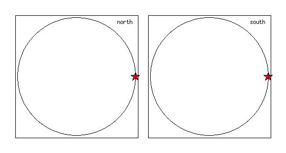X direction is

Plot of the X direction in M Tex (after setting plotx2east)

Load a check you texture

Before loading the texture, you should set your sample and crystal symmetries. In the current example, I will work with a polycrystal olivine (orthorhombic) and no special sample symmetry. I then load a VPSC texture from 60_SO_oli.tex

% Set crystal and sample symmetry
cs = symmetry('orthorhombic',[ 4.7346, 10.2149, 5.9902])
ss = symmetry('-1');

% Load the VPSC texture file
halfwidth = 10*degree;

fname = fullfile('/path/to/texture/','','60_SO_oli.tex');
ebsd60 = loadEBSD_generic(fname,'cs',cs,'ss',ss,'bunge','degree','ColumnNames',{'Euler 1' 'Euler 2' 'Euler 3' 'weight'},'header',4,'Columns',[1,2,3,4]);

You can download this texture file for testing from this link 60_SO_oli.tex.

It corresponds to the texture in a polycrystal of olivine at 60 km depth, according to the calculations presented in

Convert the texture to an ODF and plot 100 and 001 pole figures

% Create an ODF and plot a 100 and 001 pole figure, for checking
odf = calcODF(ebsd60)
plotpdf(odf,[Miller(1,0,0),Miller(0,0,1)],'contourf', 'antipodal','gray')
setcolorrange('equal');
colorbar

You should get something like this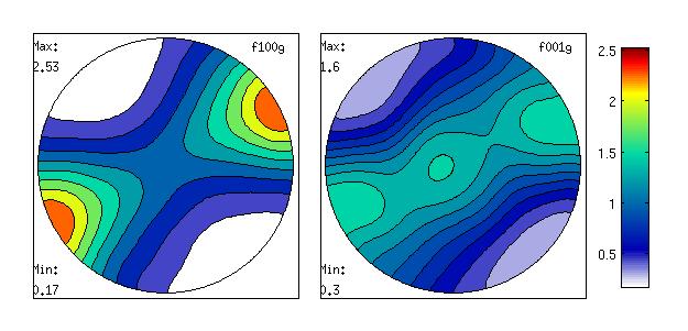

100 and 001 pole figures for our olivine polycrystal

Calculating seismic velocities

Now, we want to calculate seismic velocities for our polycrystal. You need to end the single crystal elastic moduli, density, and calculate the corresponding elastic tensor for the polycrystal. Here is how to do

% Create single crystal elastic tensor, P = 1.97 GPa, T = 1444 K
Olivine_Mat60 = ...
[[287   64   67   0.0   0.0   0.0];...
[  64  173   74   0.0   0.0   0.0];...
[  77   74  205   0.0   0.0   0.0];...
[   0.0    0.0    0.0  52   0.0   0.0];...
[   0.0    0.0    0.0   0.0  66   0.0];...
[   0.0    0.0    0.0   0.0   0.0  65]];
Cij60 = tensor(Olivine_Mat60,'name','elastic stiffness','unit','GPa', cs);
% Provide density
rho60 = 3.21
% Calculate elastic averages for the polycrystal
[ Tvoigt60 , Treuss60 , Thill60 ] = calcTensor(ebsd60, Cij60)

This will generate 3 tensors, Tvoigt60, Treuss60, and Thill60 with the elastic properties of the polycrystal in the Voigt, Reuss, and Hill average.

Plotting compression wave velocities

Here is an example for plotting compression wave velocities

plot (Thill60,'PlotType' , 'velocity' , 'vp' , 'complete', 'density' , rho60 )
axis off
box off
colorbar
title('Vp (km/s) - 60 km')

You will get a figure like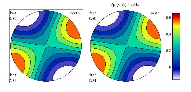

Compression wave velocities for our olivine polycrystal

If, for some reason, you want to fix the contours yourself, this is how you do

plot (Thill60,'PlotType' , 'velocity' , 'vp' , 'complete', 'density' , rho60, 'colorRange', [7.75 8.75], 'contours', [7.75 7.95 8.15 8.35 8.55 8.75]   )
axis off
box off
colorbar
title('Vp (km/s) - 60 km - 0.2 km/s contour')

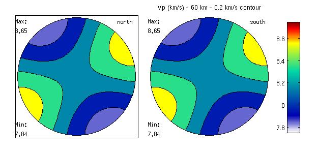Compression wave velocities for our olivine polycrystal, with contours every 0.2 km/s

Plotting shear wave anisotropy

If you want to plot the shear wave anisotropy, in percent, use

plot (Thill60,'PlotType' , 'velocity' , '200*(vs1-vs2)./(vs1+vs2)' , 'density' , rho60 )
axis off
box off
colorbar
title('dVs (%) - 60 km')

Shear wave anisotropy for our olivine polycrystal

If, for some reason, you want to fix the contours yourself, this is how you do

plot (Thill60,'PlotType' , 'velocity' , '200*(vs1-vs2)./(vs1+vs2)' , 'density' , rho60, 'colorRange', [0 7], 'contours', [0 1 2 3 4 5 6 7]  )
axis off
box off
colorbar
title('dVs (%) - 60 km - contours 1%')

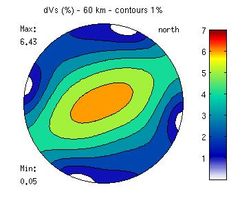Shear wave anisotropy with fixed contours for our olivine polycrystal

Plotting shear wave anisotropy, along with the direction of polarization of the fast shear wave

If you want to plot the shear wave anisotropy, along with the direction of polarization of the fast shear wave, you should use

plot (Thill60,'PlotType' , 'velocity' , '200*(vs1-vs2)./(vs1+vs2)' , 'density' , rho60)
hold all
plot (Thill60,'PlotType' , 'velocity' , 'ps1' , 'density' , rho60, 'LineWidth',2 )
hold off
box off
axis off
colorbar
title('dVs (%) - 60 km')

And here is the result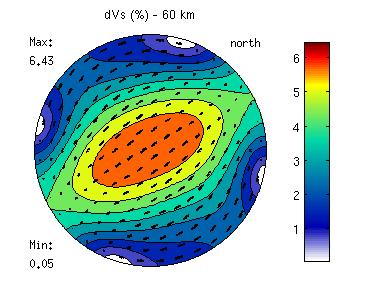

Shear wave anisotropy along with the direction of the fast polarization for our olivine polycrystal